Monte Carlo Simulation in Excel (Step-by-Step + Free Template)

Why Embrace Monte Carlo Simulation?

Traditional risk assessments often rely on single-point estimates or qualitative heat maps, which can be misleading and fail to capture the full spectrum of possibilities. monte carlo simulation in excel, on the other hand, offers a more robust approach, transforming your risk analysis Excel capabilities:

• Comprehensive Scenario Analysis: Instead of one assumption, it runs thousands of iterations, which is why it is used in schedule risk analysis and cost risk analysis simulating a wide range of possible outcomes based on defined uncertainties. This is like living the same project or operational year thousands of times, each with different assumptions and outputs.
  
  
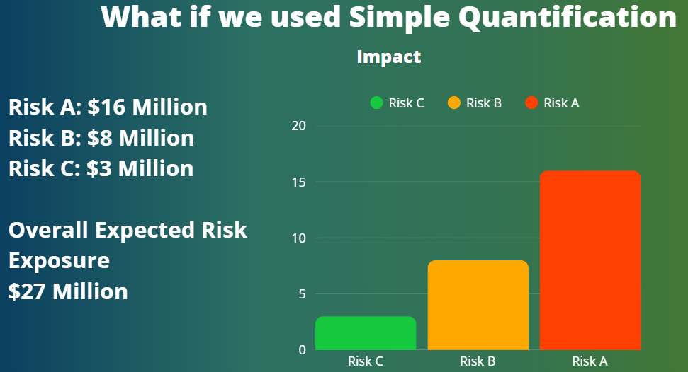
• Quantifying Risk: It allows you to move beyond vague "high," "medium," or "low" risk classifications to actual monetary values or schedule impacts. This helps you to make risk-aware decisions, backing them with evidence rather than just gut feelings.
  
  
• Contingency Planning: It helps determine the necessary contingency (e.g., budget or schedule reserves) to achieve a desired level of confidence. By using excel simulation, you gain a clear roadmap of where your project or operations are heading.

Path A: Excel Monte Carlo without add-ins (native formulas)

Works great for many project risk excel cases. You’ll use 3-point estimates (Min/Most Likely/Max) and sample with PERT/Triangular.

1) Define uncertain inputs (three-point)

Create a table: Min (A), Most Likely (M), Max (B) for each cost/duration driver.

2) Choose a distribution

• PERT (smooth, realistic for bounded tasks)

• Triangular (simple fallback when data is scarce)
  
  

3) Sample with native Excel

Tip: If the workbook gets heavy, use a Data Table or split models by area (procurement, site, commissioning).

5) Read the results

• Histogram (PDF) and S-curve (CDF) for storytelling.

• Contingency = P80 − Base (for cost); Buffer = P80 − deterministic duration (for schedule).
  
  

6) One-at-a-time sensitivity (quick tornado)

Create a small table of Low (−10%) / High (+10%) shocks on top inputs, capture the output delta |High−Low|, sort desc, and chart as a stacked bar. That’s your tornado—and the backbone of your mitigation plan.

⚠️ Correlation: Native Excel has no simple correlation sampler. If co-movement matters (e.g., shared subcontractor across tasks), consider Path B (add-ins) or rank-order correlation methods (advanced).

Path B: Step-by-Step Tutorial: Performing Monte Carlo Simulation in Excel

Here's how to run Monte Carlo in Excel, typically using an add-in like Argo (a free tool) or ModelRisk (a commercial one), as direct excel monte carlo without add-ins It runs thousands of iterations, which is why it’s used in Schedule Risk Analysis and Cost Risk Analysis:

Step 1: Identify Uncertain Inputs

All risk models begin by identifying the uncertain inputs. For risk events, these primarily include:

• Probability or Frequency: How likely is the event to occur, or how many times might it occur within a specific period?.
• Impact: What would be the consequence if the event occurs (e.g., cost, time, reputation)?

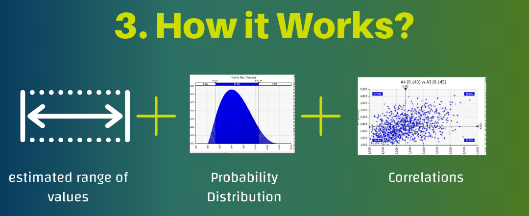
Step 2: Define Estimated Range of Values

For each uncertain input, define a range of possible values. This could be a minimum, most likely, and maximum value. For instance, for groceries, this could be the minimum, most likely, and maximum quantity or unit cost.

Step 3: Select Appropriate Probability Distributions

This is crucial for representing the nature of your uncertainties. Excel simulation add-ins provide a variety of distributions:

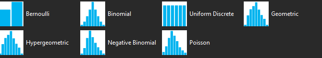
• Bernoulli Distribution: Represents a single event that either occurs or does not (binary, on/off). For example, whether a specific truck breaks down.
• Binomial Distribution: Used for multiple independent events of the same nature, each with the same probability of success/failure. Useful for scenarios like multiple trucks breaking down.
• Poisson Distribution: Models the number of times an event occurs over a fixed period (frequency). Examples include the number of claims in medical insurance or equipment breakdowns per year. The average frequency is often called the lambda factor.

• Discrete Uniform Distribution: Assigns equal probability to a finite set of distinct outcomes, often used when you have a set of distinct options with equal likelihood, like a dice roll.

• Continuous Probability Distributions: Used for outcomes that can take any value within a range.
  

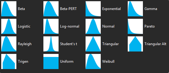
• Uniform Distribution: Often called the "clueless distribution", used when you only know the minimum and maximum values, assuming all values in between have an equal chance of occurring.
• Triangle Distribution: Requires a minimum, most likely (mode), and maximum value. It's useful when data is insufficient but you have some informed guesses and tends to provide a more conservative result than PERT.
• PERT Distribution: Similar to Triangle but with a smoother, bell-shaped curve, often used when you have higher confidence in your three-point estimates (minimum, most likely, maximum).
• LogNormal Distribution: A highly realistic distribution, especially in financial and operational risk, as it accounts for long-tail events or "fat tails"—scenarios where extreme, low-probability events can have a very high impact. It never provides negative values, which is suitable for costs or durations. It can also be defined by an expected loss (EL) at P50 and an ultimate loss (UL) at P95 or P99, representing extreme scenarios.
• Normal Distribution: Often called the "mother of distributions", it represents natural phenomena where values cluster around a mean (bell curve). It's defined by a mean (mu) and a standard deviation (sigma), where standard deviation indicates the spread or uncertainty. It's also frequently the output shape of Monte Carlo simulations.

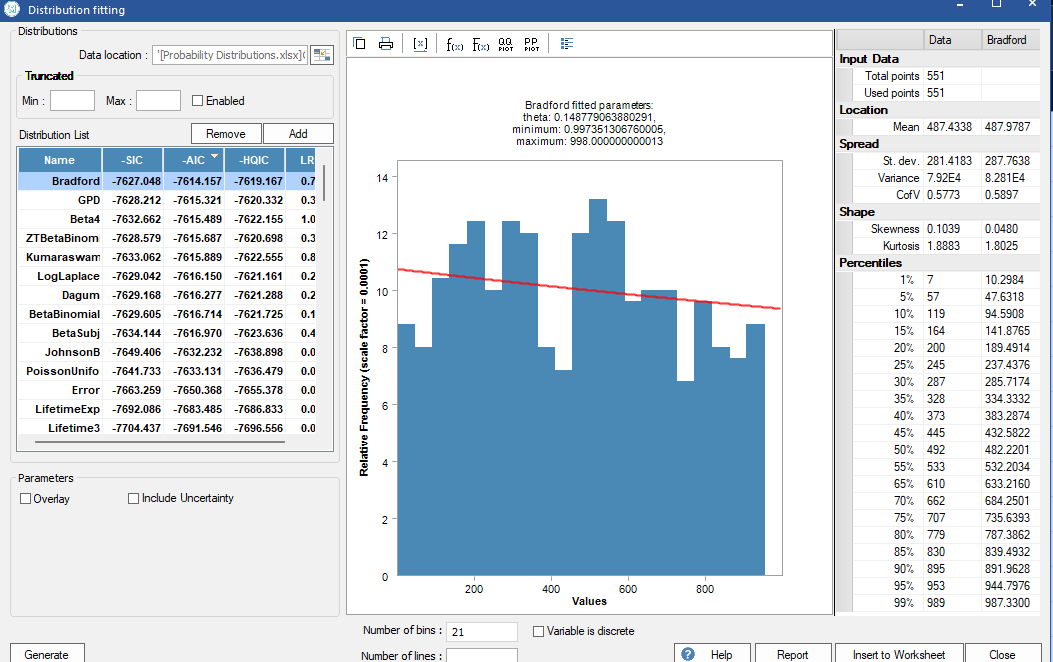
Distribution Fitting: If you have historical data (e.g., from a Risk Data Engine - RDE), tools like ModelRisk can automatically fit the best probability distribution to your data points using statistical criteria.

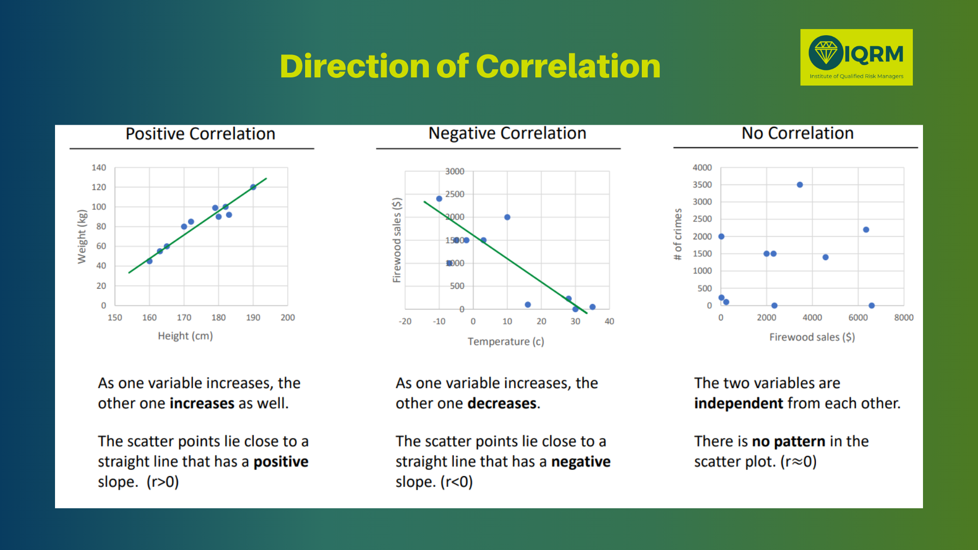
Step 4: Include Correlation (Optional but Recommended)

Correlation models the relationships between different inputs. For example, if two activities are performed by the same subcontractor, their performance might be correlated. Ignoring correlations can lead to unrealistic results; positive correlation increases overall uncertainty, while negative correlation can reduce it.

Step 5: Run the Simulation (Iterations)

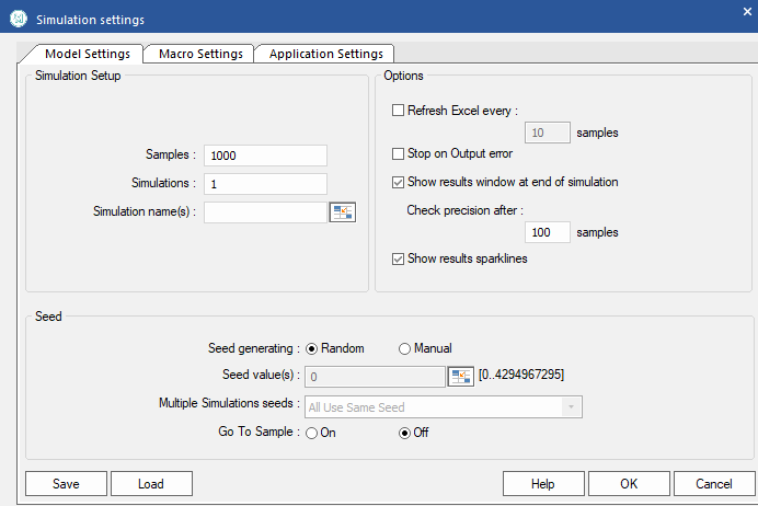
Once inputs, ranges, distributions, and correlations are set, run the simulation. This involves performing thousands of iterations (e.g., 1,000, 5,000, or 10,000).

• Lock the Random Seed: Crucial for consistency. By setting a fixed seed value (e.g., 0 or 1), you ensure that every time you run the simulation, you get consistent results for comparison.
• Stop at Convergence: For very large and complex models, this option allows the simulation to stop early once a certain level of accuracy (e.g., 97% confidence with 3% tolerance for the mean, P20, P50, P80) is reached, saving computational time without compromising results.
• Latin Hypercube Sampling: An alternative sampling method that can speed up simulations for large models by splitting iterations into "bins".
  
  

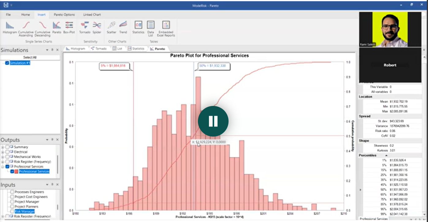
Step 6: Analyze Outputs

The output of a Monte Carlo simulation provides rich insights:

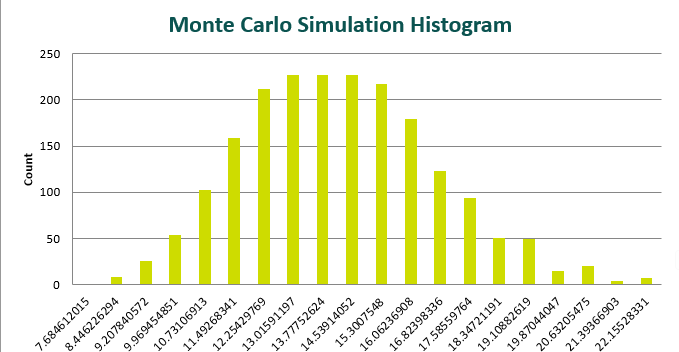
• Probability Density Chart (PDF): A histogram showing the frequency or probability of different outcomes. The x-axis represents the values (e.g., budget, duration), and the y-axis represents the probability or frequency of those values occurring.
  

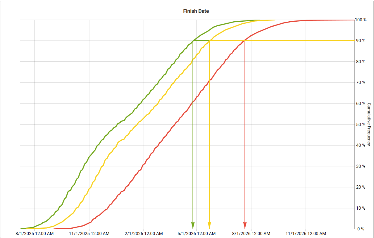
• Cumulative Density Function (CDF) / S-Curve: This curve displays the cumulative probability of outcomes. It allows you to determine the probability of achieving a certain value or identifying a value for a specific confidence level (e.g., P80 or P90). For instance, P80 means there's an 80% chance the outcome will be less than or equal to that value, and a 20% chance it will exceed it. This is vital for setting realistic contingencies.
  

• Statistics:
  • Mean (Average): The average expected value of all simulated outcomes.
  • Standard Deviation: Measures how much the results deviate from the mean, indicating the level of uncertainty or risk. A higher standard deviation means more uncertainty.
  • Percentiles: Specific points on the CDF curve (e.g., P5, P50, P80, P90, P95) that indicate the value below which a certain percentage of outcomes fall.
    
    
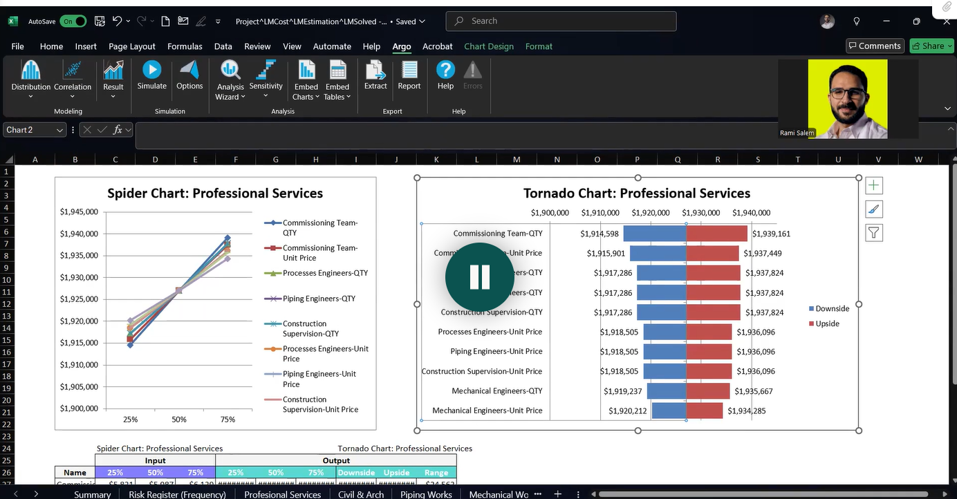
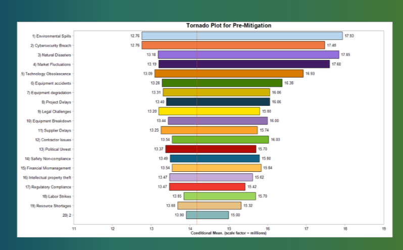
• Tornado Chart: Ranks the input variables by their impact on the overall output. It helps identify the most critical risks and uncertainties that require focused attention for mitigation or control.
  
  

How to Apply Monte Carlo Simulation in Excel

While specialized software like ModelRisk or Safran Risk offer advanced features, you can start with monte carlo in excel using a free add-in like Argo.

1. Install Argo: Download Argo from its official source. In Excel, go to File > Options > Trust Center > Trust Center Settings > Trusted Locations, and add the folder where Argo is installed. Then, enable Argo as an Excel add-in.
2. Define Inputs: In your Excel sheet, identify cells for quantities, unit prices, or other variables. Instead of single values, you will use Argo's distribution functions (e.g., ArgoTriangle(min, most likely, max) or ArgoUniform(min, max)) in these cells.
3. Combine Inputs: Multiply probabilistic quantities by probabilistic unit costs to get a probabilistic total for each item. Use the SUM function to aggregate these totals for an overall project cost or duration.
4. Define Outputs: Mark the aggregated total (e.g., total project cost) as an output in Argo.
5. Run Simulation: Use Argo's simulation settings to define the number of iterations and ensure the random seed is locked for consistent results.
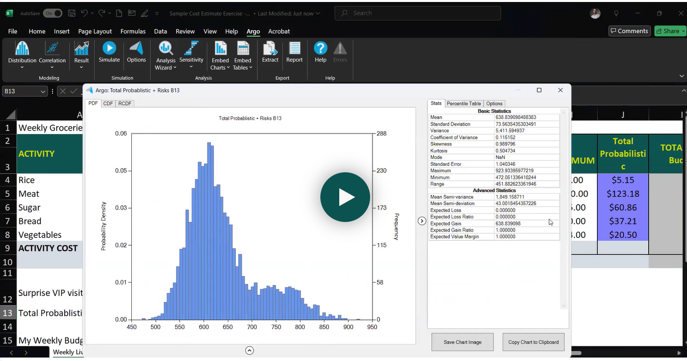
6. Analyze: Use Argo's analysis wizard on your output cell to view the PDF, CDF, and statistics, gaining insights into your project's risk profile.
   
   

Presenting Results for Impact

Effective communication is key for decision-makers to buy into your analysis.

• Keep it Simple: Avoid overwhelming with too many charts or excessive decimal places.
• Use Visuals Strategically: Tornado charts are excellent for showing risk rankings clearly. CDF curves can illustrate confidence levels like P80 or P90.
• Tell a Story: Frame your analysis as a narrative, linking data to actionable insights. For example, "We are exposed to $180K of losses if concrete trucks fail, so we recommend securing a secondary supplier at $5K".
• Focus on Actionable Recommendations: Clearly state what decisions need to be made and what the impact of those decisions will be.
  

Free Template!

To help you get started with your project risk Excel analysis, I'll share an Excel sheet similar to the one discussed in this tutorial. You can use this excel monte carlo template to practice applying these concepts to your own personal expenses, project estimates, or any other area where you need to manage uncertainty. This hands-on practice is invaluable for truly understanding Monte Carlo Simulation and its benefits.

By leveraging Monte Carlo Simulation in Excel, you can transform the way you assess and manage risk, moving from guesswork to data-backed, confident decision-making.