Key Takeaways
-
Import Primavera P6/Microsoft Project → fix constraints/open ends/long lags before simulating.
-
Separate inherent uncertainty from discrete risk events; use calendar risks for seasonality/weather.
-
Enable Latin Hypercube Sampling and Stop at Convergence for stable P50/P80/P90 results.
-
Use drivers/sensitivity to target mitigations and quantify pre → post improvements.
-
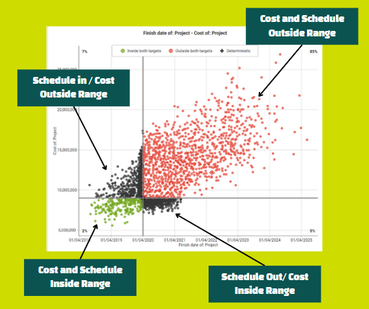
Integrate cost to present JCL (probability of meeting time and budget together).
Glossary
QSRA: Quantitative Schedule Risk Analysis.
P-date: Percentile completion date (e.g., P80).
JCL: Joint Confidence Level (probability to hit time & cost together).
LHS: Latin Hypercube Sampling.
Calendar risk: Time-dependent downtime windows (e.g., monsoon, sandstorms).
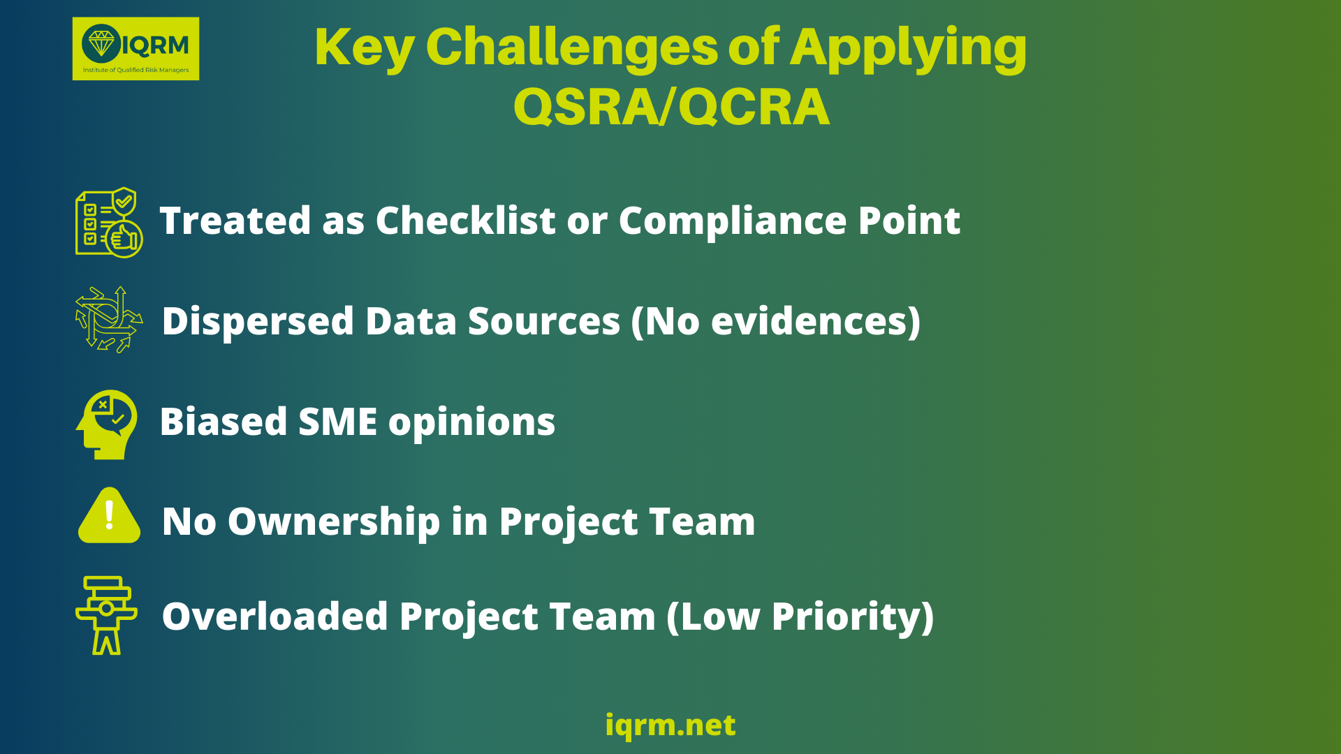
Why traditional schedule risk analysis (QSRA) often underdelivers:
-
Lack of diligence: QSRA done for compliance, not decisions.
-
Dispersed, unsubstantiated data: weak evidence behind forecasts.
-
Optimism bias: “yes” answers over realistic assessments.
-
No ownership: overloaded teams and no clear risk lead
Result: forecasts that aren’t defensible, unclear explanations for date movement, and limited visibility on what happens next.
To resolve this issues, In
QRM Diploma you will learn about something called
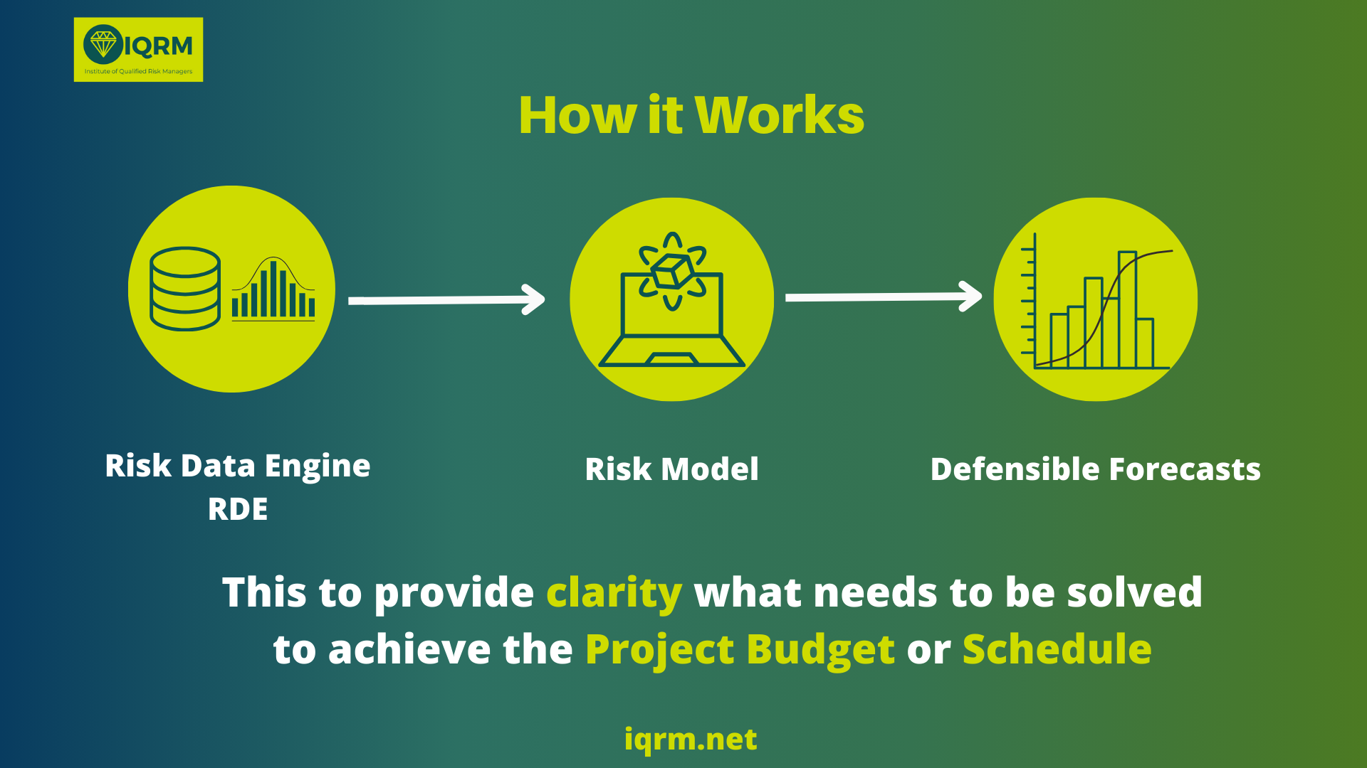
RDE or
Risk Data Engine to support So not to build schedule risk models not on Opinions, but on Data.
It is a systematic way to collect and study data to provide the best data driven information to the Schedule Risk Model with minimum amount of bias from the SME to Support the Schedule Risk Analysis process.
Safran Risk operationalizes a is data-driven schedule risk analysis:
-
Structured ingestion & checks: Import from P6/MS Project; run schedule warnings to make the network simulation-ready.
-
Fit-for-purpose simulation: Monte Carlo with Latin Hypercube Sampling and Stop at Convergence for speed and stability on large models.
-
Scenario clarity: Toggle pre- vs post-mitigation to quantify improvement in days at your decision percentile.
-
Decision alignment: Integrate cost with schedule to communicate JCL clearly to executives.
Step-by-step: building a schedule risk analysis model in Safran Risk
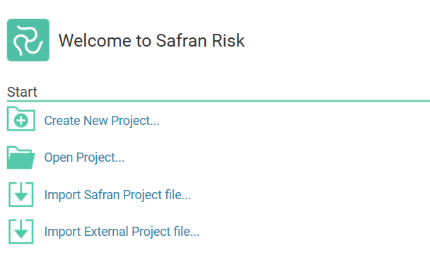
1) Import your schedule (get it “risk-ready”)
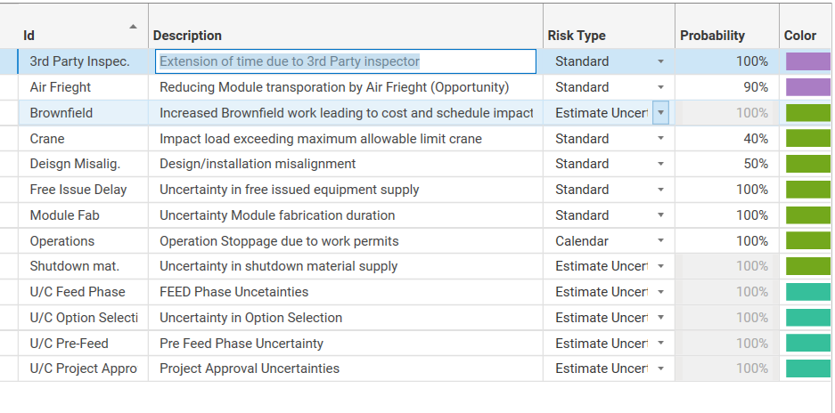
2) Define risks & uncertainties (model real behavior)
-
Standard (discrete) risks: Probability + impact; model pre/post-mitigation and include cost/duration of mitigation actions.
-
Estimated uncertainty (100% probability): bounded duration spread on activities (e.g., −20% / +50%).
-
Calendar risks: Time-dependent downtime (monsoon, sandstorm, freeze/thaw) built from templates or time-series history.
-
Non-existence risk: Simulate links/activities that may or may not exist (permits, optional scope).
-
Probabilistic branching: Competing paths (e.g., shallow vs deep foundations) with branch probabilities.
-
Global risks: Standardize reusable risks as an organizational template; import/export via Excel for governance.
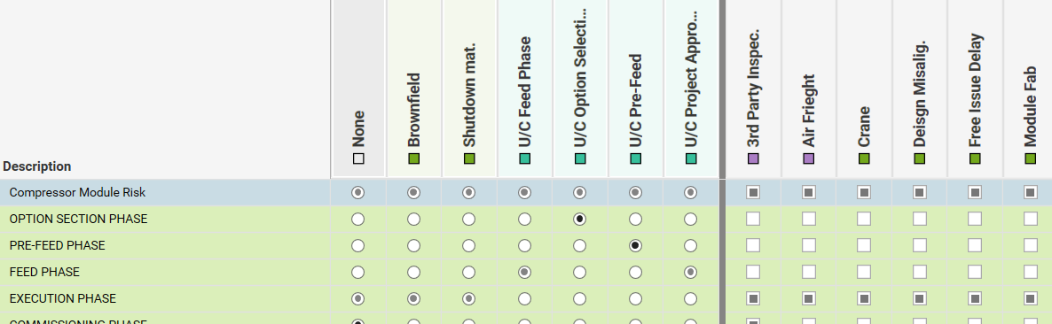
3) Map risks to the right work (where it truly bites)
-
Assign to activities/summaries; filter by WBS, codes, or critical path to focus effort.
-
Series vs parallel impacts: Choose whether multiple risks accumulate (series) or hit concurrently (parallel).
-
Overrides: Adjust a risk’s probability/impact per activity without changing the global definition.
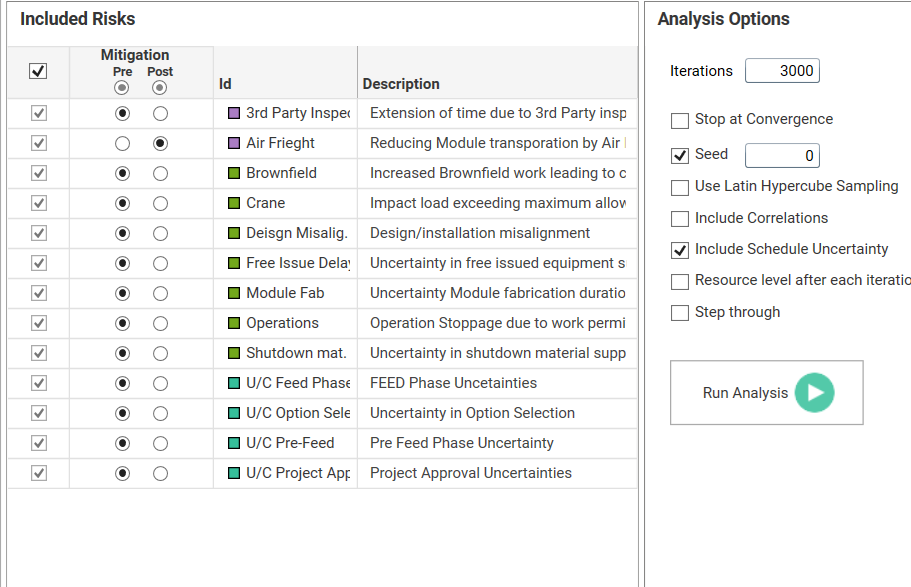
4) Configure the analysis (fast, stable, reproducible)
-
Iterations & seed: Choose iteration count and fix a seed for reproducibility.
-
Convergence: Enable Stop at Convergence with percentile targets/tolerance to end runs automatically when stable.
-
Sampling & correlation: Consider LHS and include correlations where defined.
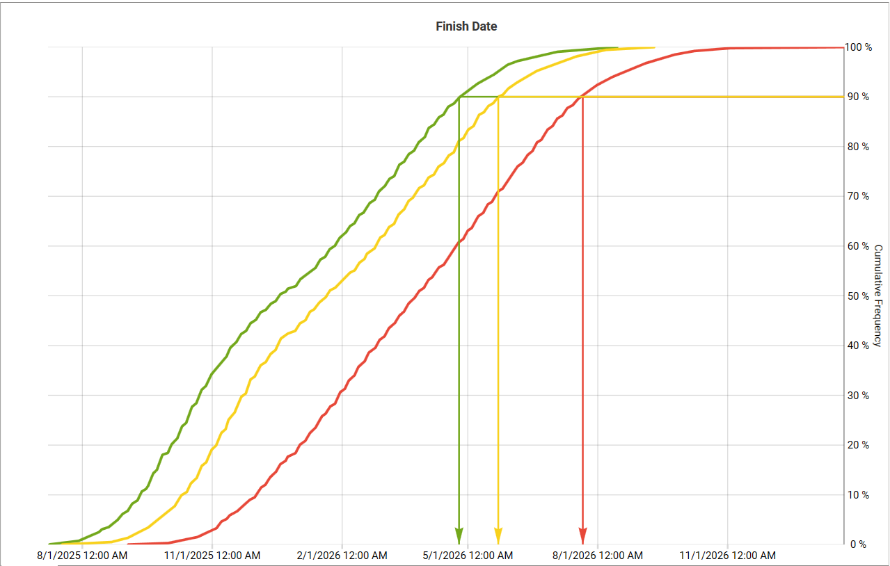
5) Read the results like a decision-maker
-
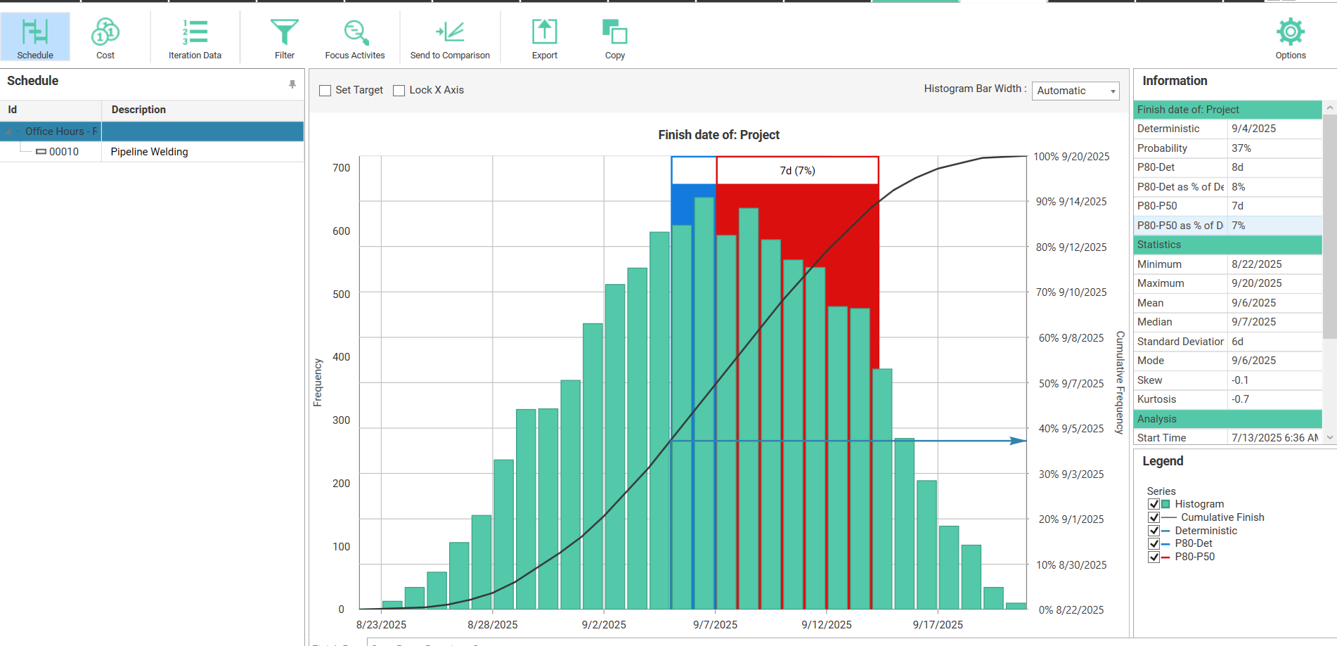
Distributions & P-dates: Report mean/median and P50/P80/P90; add visual curtain annotations at decision percentiles.
-
Drivers & sensitivity: Use tornado/driver views to identify where contingency truly comes from.
-
Compare scenarios: Show days of improvement (e.g., “71 days improvement”) from pre → post mitigation; keep artifacts for audits.
-
From P-dates to actions: Tie the top drivers to targeted mitigations and update the plan and baseline appropriately.
Integrate cost & schedule: move to Joint Confidence Levels (JCL)
When timing and money both matter (always), integrate cost with your schedule risk analysis to produce JCL, the probability of achieving both targets simultaneously (e.g., meet the date and budget at P80). This is the language executives understand.
Schedule risk analysis checklist
FAQs
Q1) What is schedule risk analysis in practice?
A simulation-based approach (QSRA) that quantifies uncertainty and discrete risks on a project schedule, producing P-dates and drivers so decisions reflect reality, not optimism.
Q2) Can I use Safran Risk with Primavera P6 or Microsoft Project?
Yes—import your plan, then resolve schedule warnings (constraints, open ends, long lags) to ensure realistic simulation outputs.
Q3) Why use calendar risks instead of just widening duration ranges?
Calendar risks capture time-dependent downtime (e.g., monsoon periods) that duration ranges alone cannot represent accurately.
Q4) Should I enable Latin Hypercube Sampling (LHS)?
LHS often improves coverage of input distributions and can speed convergence. Use with convergence controls for large models.
Q5) How do I prove mitigation works?
Model pre/post states and use distribution comparison to quantify improvement in days at your decision percentile (e.g., P80).
Ready to master schedule risk analysis end-to-end?
Join the Schedule Risk Analyst Course (Safran Risk edition) and learn how to:
-
Import & health-check P6/MSP schedules (constraints, lags, open ends)
-
Model uncertainty, discrete risks, calendar risks, and probabilistic branching
-
Configure simulations with LHS + convergence for stable P50/P80/P90
-
Pinpoint delay drivers (tornado), prove pre→post mitigation impact, and communicate JCL
-
Ship audit-ready QSRA deliverables your executives actually use.
Who it’s for: Planners, Schedulers, Risk Engineers, PMO, Cost Controllers.
Includes: Practical case exercises.