Cost Risk Analysis and Contingency: How to Size It with Data
Most project teams size contingency by guessing. A project director picks a round number, say 10% or 15%, based on experience, gut feel, or what the budget can absorb. The result? Either too much money locked up doing nothing, or not enough to cover the risks that actually materialize.
Cost risk analysis (also called Quantitative Cost Risk Analysis or QCRA) is the process of using Monte Carlo simulation to stress-test a project budget and determine a data-driven project contingency at a specific confidence level, typically P80. It replaces percentage-based guesswork with a defensible number backed by probabilistic modelling, giving decision-makers a clear view of budget risk and potential cost overrun exposure.
Cost risk analysis replaces this guesswork with a defensible, data-driven number. Instead of asking "what percentage feels right?", you run a probabilistic cost estimate that tells you exactly how much contingency you need, and at what confidence level.
Here is how it works, step by step.
What Is Cost Risk Analysis?
Cost risk analysis, also known as Quantitative Cost Risk Analysis (QCRA), is the process of stress-testing a project budget using Monte Carlo simulation. It takes your deterministic base estimate, the single-number budget from your cost engineers, and runs it through thousands of simulated scenarios. Each scenario applies different combinations of cost uncertainties and risk events to show the full range of possible outcomes.
The output is not a single number. It is a probability distribution that shows the likelihood of completing the project at or below any given cost. This is the fundamental shift from deterministic to probabilistic estimation: you move from "the project will cost $120 million" to "there is an 80% chance the project will cost $135 million or less."
Why Percentage-Based Contingency Fails
The traditional approach to contingency is to add a flat percentage on top of the base estimate. This method has three critical problems that increase budget risk and expose projects to cost overrun.
First, it ignores the actual risk profile of the project. A 10% contingency on a straightforward civil works package is very different from 10% on a complex brownfield turnaround.
Second, it cannot be defended under scrutiny. When a project director asks "why 15% and not 12%?", there is no analytical answer.
Third, it gives no insight into what is driving the cost uncertainty. Without understanding which cost elements carry the most risk, mitigation efforts become unfocused and reactive.
The QCRA Process: From Base Estimate to Defensible Contingency

Step 1: Start with the Deterministic Base Estimate
Every cost risk analysis begins with the base cost estimate produced by quantity surveyors or cost estimators. This is the planned budget with quantities and unit rates for each project element.
Step 2: Define Business-as-Usual Uncertainties
These are systemic cost uncertainties that exist on every project. They have a 100% probability of occurring, because no estimate is perfectly accurate. Apply continuous probability distributions (Triangle or PERT) to define minimum, most likely, and maximum ranges for Quantities and Unit Prices.
Step 3: Identify and Quantify Discrete Risk Events
Specific contingent events may or may not occur: equipment damage, sudden inflation spikes, regulatory changes. Each risk event is assigned a probability of occurring and a cost impact range. These are modeled as discrete risks with conditional distributions.
Step 4: Link Cost to Schedule (For Integrated Models)
In advanced QCRA, cost and schedule are connected. Variable costs are mapped to activity durations using time-dependent cost rates, so delays automatically increase cost. This produces a Joint Confidence Level (JCL) that captures the true project exposure.
Step 5: Run Monte Carlo Simulation
The Monte Carlo engine runs 5,000 to 10,000 iterations, aggregating all uncertainties, risk events, and correlations into a probability distribution of total project cost. For a hands-on walkthrough, see our guide: Monte Carlo Simulation in Excel (Step-by-Step).
Step 6: Read the Outputs and Size Your Contingency
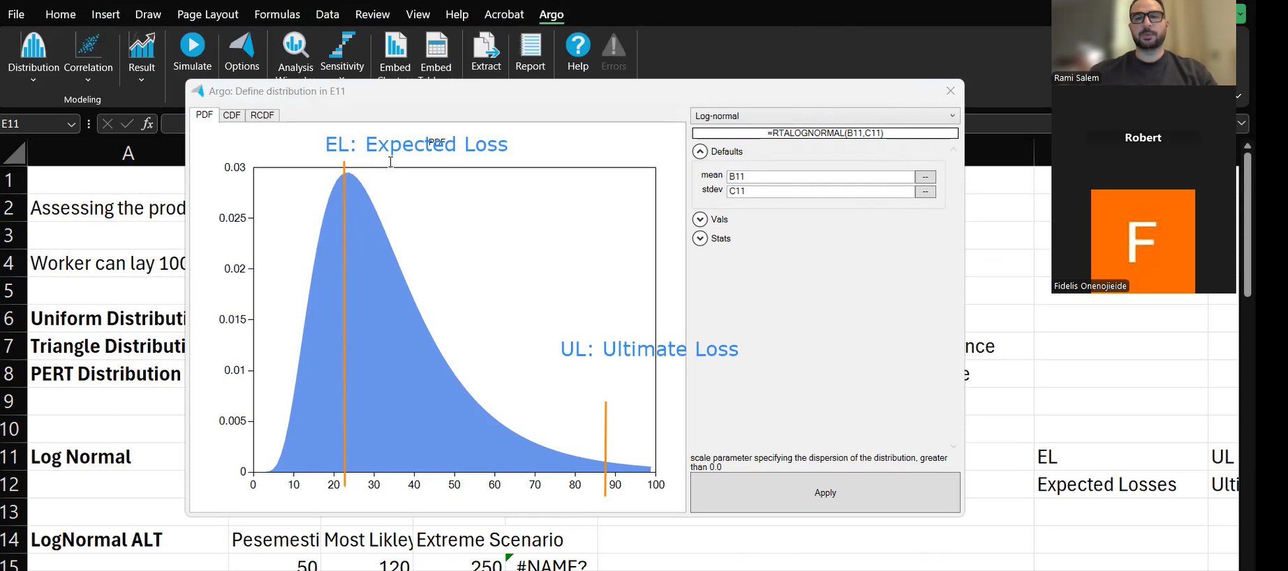
The Histogram (PDF): Shows the frequency distribution of possible cost outcomes.
The S-Curve (CDF): The decision-making tool showing cumulative probability of achieving any given cost.
Cost Contingency = P80 Cost - Deterministic Base Estimate
If your base estimate is $120 million and the P80 cost is $135 million, your data-driven contingency is $15 million. Not a guess. A calculated, defensible figure.
Step 7: Identify Cost Drivers with Tornado Charts
The tornado chart ranks every variable and risk event by how much variance it injects into the total cost. This sensitivity analysis shows exactly where risk is concentrated and where mitigation will have the biggest impact.
Step 8: Separate Contingency from Management Reserve
Contingency covers quantified risks. Management reserve covers unknown unknowns. These two should never be blended in your project contingency framework. A properly sized contingency from QCRA gives you a defensible number for known risks. Management reserve is a governance decision, not a modeled output.
Choosing the Right Confidence Level: P50 vs P80 vs P90

| Confidence Level | Description | Typical Use |
|---|---|---|
| P50 | 50% confidence (median) | Aggressive target, contractor bid pricing |
| P80 | 80% confidence (industry standard) | Project planning, contingency sizing |
| P90 | 90% confidence (conservative) | High-stakes, regulated environments |
A Real-World Scenario
Consider a brownfield turnaround in the GCC with a base estimate of $200 million. Traditional contingency at 10% would set aside $20 million.
After QCRA:
P50 cost: $218 million
P80 cost: $237 million
P90 cost: $251 million
Data-driven contingency at P80: $37 million -- nearly double the percentage-based guess.
Without the analysis, the team would have been $17 million short at P80.
Best Practices for Effective Cost Risk Analysis
Separate quantity risk from unit rate risk. They compound differently. A 10% increase in both creates a 21% cost increase, not 20%.
Model indirect costs as time-dependent. Linking them to schedule durations captures the real cost of delays.
Use correlation between related cost elements. Steel and rebar prices tend to move together.
Present contingency as a calculated number, not a markup.
Run pre-mitigation and post-mitigation scenarios. Show the impact of your risk response plan on the S-curve.
From Guesswork to Governance
Cost risk analysis is not an academic exercise. It is a governance tool that transforms how organizations allocate budgets, approve projects, and protect delivery budgets.
The methodology is proven. The tools are available. The question is whether your organization is still sizing contingency by gut feel, or by data.
Frequently Asked Questions
What is the difference between cost risk analysis and a risk register?
A risk register lists identified risks qualitatively. Cost risk analysis takes those risks, assigns probability distributions and cost impacts, and models them through Monte Carlo simulation to produce a quantified cost forecast. The register is the input. The analysis is the output.
What software is used for Quantitative Cost Risk Analysis?
Common tools include Safran Risk, @Risk (Palisade), and Crystal Ball. For integrated cost-schedule models, Safran Risk is widely used in the oil and gas, infrastructure, and EPC sectors. Excel-based models with Monte Carlo add-ins are also common for simpler analyses.
What confidence level should I use for contingency: P50, P80, or P90?
P80 is the industry standard for project planning and contingency sizing. P50 is used for aggressive contractor targets. P90 is reserved for high-stakes or regulated environments. The right level depends on your organization's risk appetite and governance requirements.
How many Monte Carlo iterations are needed for reliable results?
A minimum of 5,000 iterations is standard practice. Most professionals run 10,000 iterations to ensure convergence. Running fewer than 1,000 produces unreliable outputs with significant statistical noise.
Can cost risk analysis be done without schedule integration?
Yes. A standalone QCRA models cost uncertainties and discrete risks without linking to schedule. However, for projects where time-dependent costs (like site overheads or equipment rental) are significant, integrated cost-schedule analysis produces more accurate results.
IQRM delivers specialist training and consulting in Quantitative Cost Risk Analysis, Monte Carlo simulation, and risk-based forecasting. Our QRM Diploma programme equips professionals with the practical skills to build, run, and interpret cost risk models on real projects.
Frequently asked questions
What is cost risk analysis in project management?
How do you calculate contingency using Monte Carlo simulation?
What confidence level should I use for contingency: P50, P80, or P90?
How many Monte Carlo iterations are needed for reliable results?
Can cost risk analysis be done without schedule integration?