Schedule Risk Analysis: Complete Guide with Monte Carlo & Examples

Schedule Risk Analysis (SRA), often called Quantitative Schedule Risk Analysis (QSRA), uses Monte Carlo simulation to quantify how uncertainty and discrete risks affect your project dates.

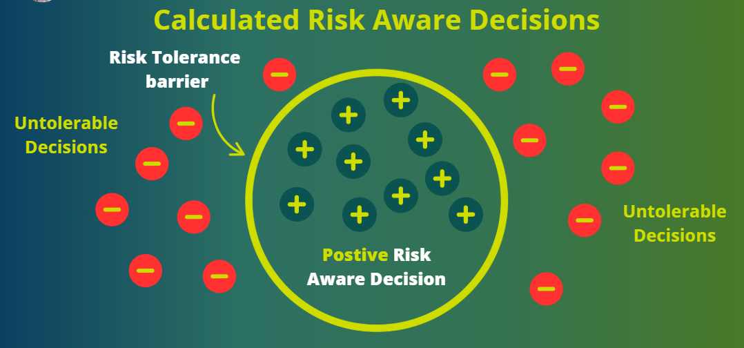
Instead of one optimistic finish date, QSRA gives you a distribution of outcomes (P50/P80/P90) and shows which risks and activities drive delay, so you can size buffers and make risk-aware decisions.

Why schedule risk analysis matters

• Better decisions: Replace gut feel with evidence (P-values, drivers, confidence).

• Realistic forecasts: Know the probability of hitting key milestones/finish date.

• Right-sized buffers: Derive schedule contingency from P-values, not padding.

• Targeted mitigation: Identify top risk drivers and critical activities to act on.

Key concepts 

1) Discrete risks vs. inherent uncertainty

• Risk events (discrete/contingent): May or may not occur (<100% probability). Example: crane breakdown, permit delay.

• Estimated uncertainty (inherent/systemic): Always present (100% probability) but range-based (e.g., −20% to +50% of planned duration). Typically one duration-uncertainty per activity in tools like Safran Risk, applied independently across activities.

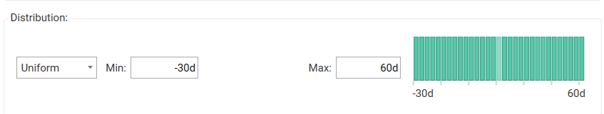
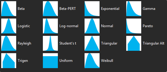
2) Probability distributions (when to use what)

• Triangular: Min/Most-Likely/Max with scarce data; transparent and simple.

• Beta-PERT: Smoothed version of triangular for bounded durations/costs.

• Lognormal: Positive-only with long tails (common for overruns/costs).

• Normal: Symmetric; useful for aggregated effects, less so for bounded tasks.

• Bernoulli / Binomial / Poisson: For discrete on/off events or event frequency.
  

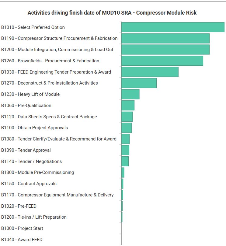
3) Drivers, criticality, and sensitivity

• Risk drivers: Risks that contribute most to delay (rank via tornado charts).
  

• Activity drivers: Tasks most frequently on the path that moves the finish.

• Criticality index: % of simulations where an activity is on the critical path.

Schedule risk analysis steps (end-to-end)

Step 1 — Prepare the schedule (import & health checks)

• Import: Bring Primavera P6 XER or Microsoft Project MPP/XML into your SRA tool (e.g., Safran Risk or Primavera Risk Analysis). Confirm planning units (hours vs days).

• Schedule warnings:

  • Constraints: Replace hard date constraints (MFO/MSS) with logic wherever feasible—constraints distort stochastic behavior.

  • Open ends: Close tasks lacking predecessors/successors (except start/finish).

  • Long lags/leads: Convert to dummy activities so you can apply uncertainty/risks explicitly.

  • Hammock/soft logic: Avoid SS/FF overuse that “stiffens” networks and hides drivers.

Document accepted warnings and why you kept them—this builds auditability.

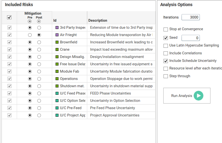
Step 2 — Identify & quantify risks (build the risk register)

• Write clear risk statements (Why cause → What event → How effect).

• Quantify probability/frequency and impact ranges (days/$).

• Capture pre-mitigation and post-mitigation states (with action cost/duration).

• Maintain owners, due dates, evidence, and data sources (supports governance).
  
  

• Pro-tip: create global risks templates for recurring items (weather, interfaces).

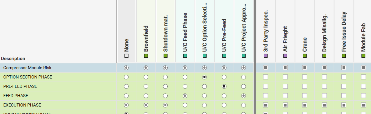
Step 3 — Map risks to activities (where it truly bites)

• Assign one duration-uncertainty per activity; add multiple discrete risks as needed.

• Define interaction logic: Series (impacts add up) vs Parallel (impacts occur concurrently; overall impact is the largest). Most mappings are Series.

• Apply overrides per activity if a global risk behaves differently on a specific task.

• (Advanced) Add correlations where drivers are linked (shared crews, locations).
  

Step 4 — Configure Monte Carlo simulation

• Iterations: 5,000–10,000 for stable tails (more for critical portfolios).

• Seed: Lock a random seed for reproducibility in reviews.

• Convergence: Enable “stop at convergence” to end runs once results stabilize (saves time).

• Sampling: Consider Latin Hypercube Sampling (LHS) for even coverage.

• Include schedule uncertainty and defined correlations if modeled.
  

Step 5 — Analyze results & compare scenarios

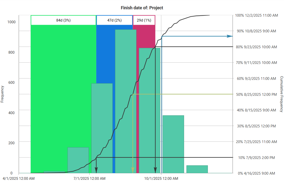
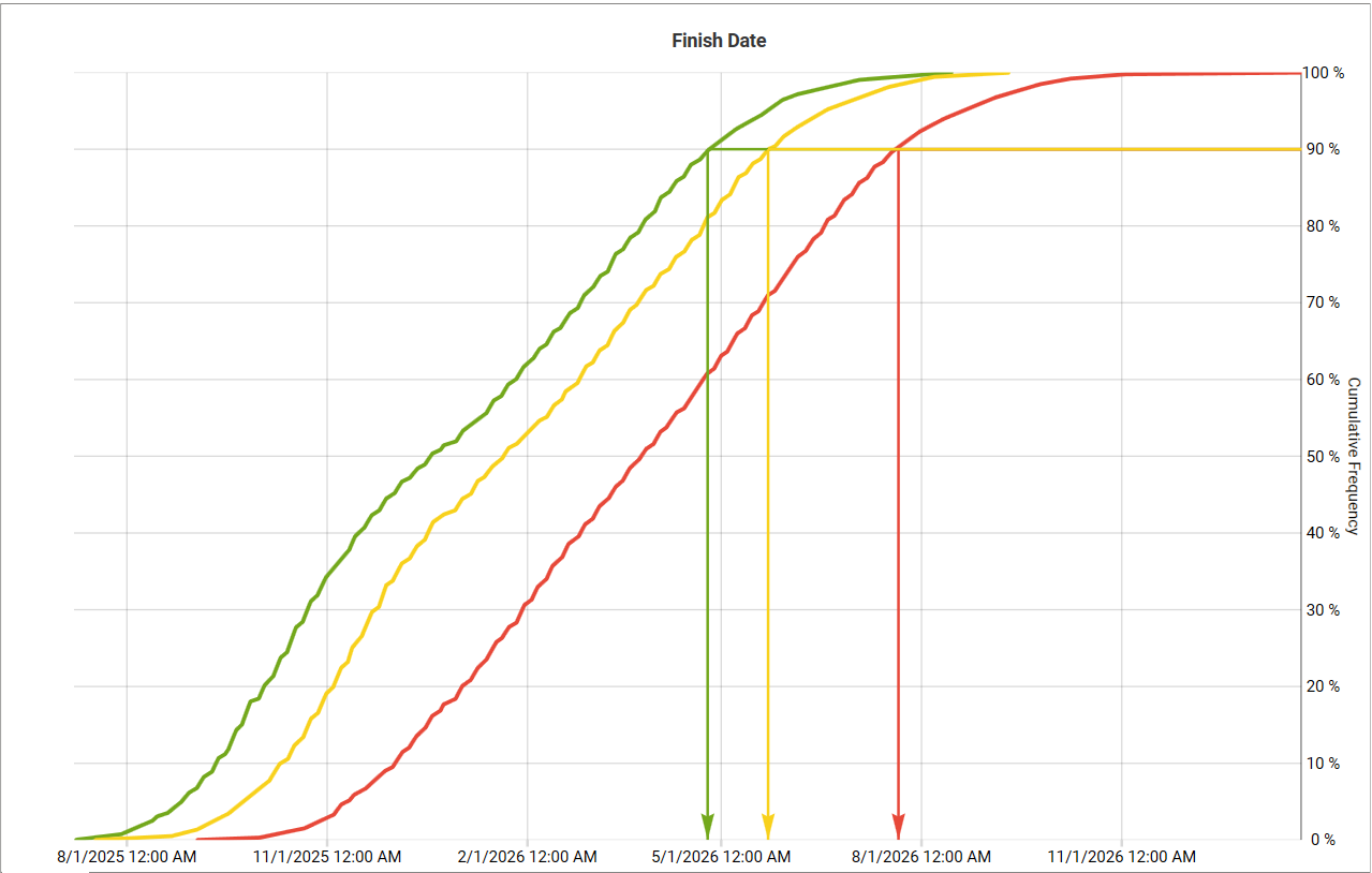
• Distribution & P-dates: Read mean/median plus P50/P80/P90 on finish and key milestones (add visual “curtains” at decision percentiles).

• Sensitivity (tornado): Rank top delay drivers—these become your action list.

• Criticality/path analysis: See which activities frequently drive the finish.

• Pre vs post mitigation: Quantify improvement (e.g., “71 days earlier at P80”).

• Convert P-dates to buffers (and, when cost is integrated, to JCL decisions).
  

Step 6 — Report & act (make it stick)

• Lead with a one-liner: “At P80, finish = 17 Nov 2026 (buffer +38d).”

• Show S-curve + tornado; list 3–5 prioritized actions with owners/dates.

• Update monthly/quarterly: keep register and mappings current; trend P-dates.

Tools you can use

• Safran Risk: Specialized for schedule, cost, and integrated risk; strong import checks, mapping, correlations, convergence, driver analysis, and reporting.

• Primavera Risk Analysis (Pertmaster): Oracle ecosystem option for schedule/cost risk.

• Excel + add-ins (e.g., Argo/ModelRisk): Good for prototypes and pedagogy; supports PDFs/CDFs and sensitivity; heavier models benefit from dedicated tools.

QSRA best practices (what separates good from great)

• Build a Risk Data Engine (RDE): Systematize data collection (internal KPIs, incident logs, supplier performance, weather/time-series). Fit distributions to data where possible.

• Calibrate expert judgment: Challenge optimism/anchoring; ask for evidence; keep most-likely and extreme cases explicit.

• Model what’s real: Use calendar risks for seasonality (monsoon, sandstorms) rather than padding durations.

• Governance: Baseline versions, naming conventions, and an approval trail for register changes and mappings.

• Align to risk tolerance: Choose P-values that match policy (e.g., plan at P50, commit at P80; safety-critical may choose P90).

Schedule risk analysis examples

Example 1: Valve procurement (pipeline)

• Risk: Long-lead control valves; global supply constraints.

• Mapping: Discrete risk on procurement + interface milestones; uncertainty on manufacturing duration.

• Result: Finish P80 = +43d vs deterministic; tornado shows procurement lead time as #1 driver.

• Action: Approve air freight for critical size valves (CAPEX +$0.4M) → P80 improves by 19d, avoids liquidated damages.

Example 2: Welding productivity (brownfield tie-ins)

• Risk: Crew absenteeism + machine failures; inherent productivity variability.

• Mapping: Uncertainty on key welding activities; discrete risks for breakdowns; mild positive correlation across similar welds.

• Result: P50 ok, but P80 breaches outage window.

• Action: Add standby machine and an extra crew on critical week → P80 moves inside the window by +12d.

Example 3 : Offshore module heavy-lift

• Risk: Weather downtime windows; fabrication rework risk.

• Mapping: Calendar risk for wind/wave thresholds; discrete rework risk on module completion path.

• Result: P90 misses crane availability window in Q4.

• Action: Pull-ahead NDE/QA and add a weather buffer; resimulate → P80 stable and P90 within window.

Call to action

Want guided, hands-on QSRA with Safran Risk (calendar risks, correlations, convergence, JCL)?
Join the QRM Diploma (Quantitative Risk Management + AI).